When we try to divide machine learning methods, we generally tend to separate them into two fundamentally different groups: supervised and unsupervised. So, where do semi-supervised methods fit in? As it is clear by the name, there is some element of supervised principles involved in this category, but what is it that makes it different from supervised learning. If I have to explain it in layman words, semi-supervised learning is a mixture of both supervised and unsupervised techniques so that we enable ourselves to make use of abundant unlabeled data to train our supervised algorithms.
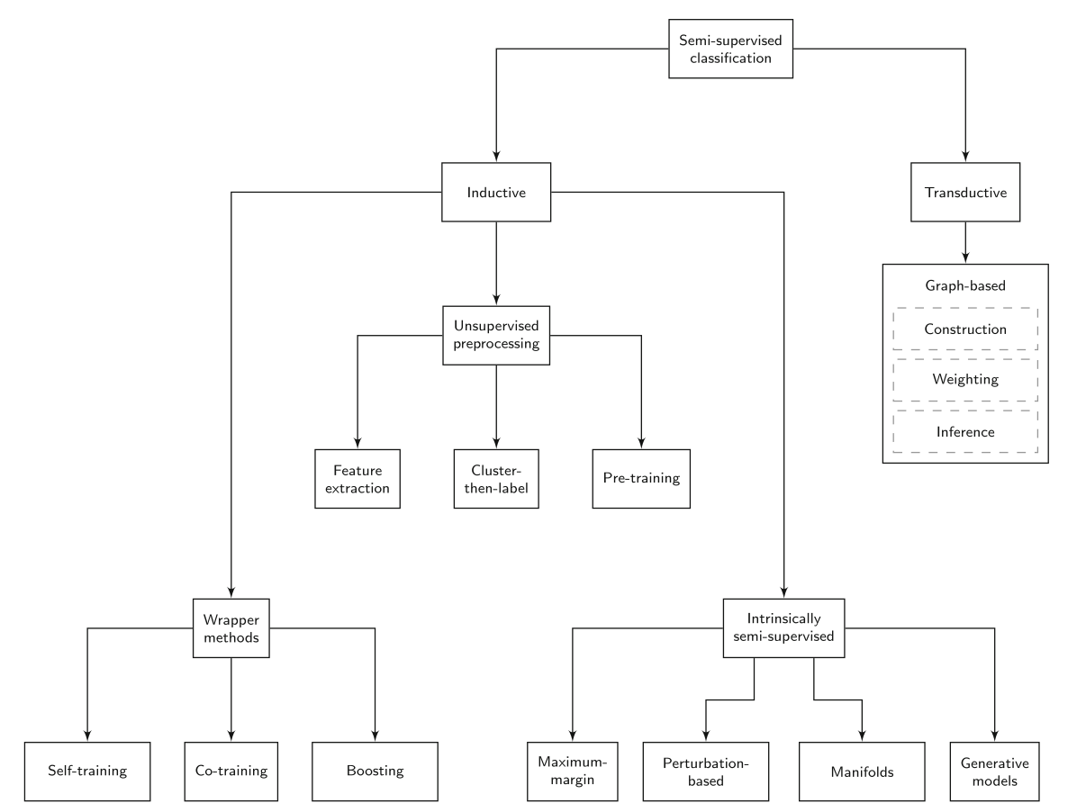
By definition, semi-supervised learning is a branch of machine learning that combines a small amount of labeled data with a large amount of unlabeled data during training to produce considerable improvement in the learning accuracy. It falls between unsupervised learning and supervised learning. The concept of semi-supervised learning is important because it allows us to prevent the cost of manually labeling the training data and make use of huge amount of unlabeled data that we can find in today’s digital world. Although, it may sound simple when we say mixing supervised and unsupervised methods is the basis of formation of semi-supervised methods, there are different ways we can approach this problem. The diagram below broadly represents the taxonomy of semi-supervised learning methods that are present to date.

Basic Concept and Assumptions
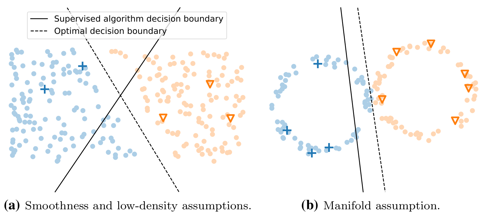
We can find unlabeled data everywhere in the form of text, images, audio signals, etc but it is very difficult to utilize them to good effect. Most of the machine learning methods (including deep learning) can only perform well only when we have properly labeled data to train the model and labeling data comes with great economic and labor cost. Semi-supervised learning methods try to make use of the unlabeled data with the help of small amount of available labeled data. But for the unlabeled data to be of any use for our algorithm, there are three main assumptions about the distribution of the unlabeled data.
Smoothness Assumption
- We assume that if two data points in the sample space are close to each other, then their labels in the output space should also be close to each other.
- Basically, if x and x’ are close, then y and y’ should also be close enough, where x is the input data and y is its label.
Low-density Assumption
- This assumption ensures that the decision boundary between classes does not pass through high-density areas, i.e. through areas where there are a lot of data points grouped together.
- It is quite intuitive that regions with higher density in sample space generally belong to a particular class and the decision boundary that separates two classes should be somewhere where almost no data are present.
Manifold Assumption
- According to manifold assumption, data points on the same low-dimensional manifold should have the same label.
- By same low-dimensional manifold, we mean the projection of data points to a lower-dimensional space using methods like Principal Component Analysis (PCA). So, if data points projected at lower dimensions are closer, then they should most probably belong to the same label or class.

The image above clarifies the different assumptions that are undertaken in almost all semi-supervised methods. In addition to these assumptions, there is one more called cluster assumption which somewhat is a generalization of all three assumptions. It states that if data points (both labeled and unlabeled) cannot be meaningfully clustered, it is impossible for a semi-supervised learning method to improve on a supervised learning method. Once these assumptions about our unlabeled data are satisfied, we can move forward to applying semi-supervised methods on the unlabeled data that we have.
Semi-supervised Learning Methods
Based on the training principle of the model, semi-supervised learning can be divided into Inductive Learning and Transductive Learning. Inductive learning refers to learning from specific (training) examples and trying to generalize the condition for the entire input space. This means in inductive learning, we try to learn a generalized function with the help of available training dataset. This generalized function may be logically true but may or may not be realistically true for every data point in the sample space. On the other hand, transductive learning is generating rules from specific training examples and then applying them to the test examples. This approach is completely domain-based and does not work for other cases of input samples. In transductive learning, we do not solve for a more general problem as an intermediate space, rather we try to get specific answer that we really need. For e.g., forming a graph with connection between similar data points through which information is propagated. This requires no training and testing phase and we do not construct a classifier for the entire input space.
Inductive Learning Methods
In these methods, a model is built in the training phase and can then be used for predicting the labels of new data points. The categories of methods that fall under inductive learning are Wrapper Methods, Unsupervised Preprocessing Methods, and Intrinsically Semi-supervised Methods which are individually explained below.
1. Wrapper Methods
The principle behind wrapper methods is that we train a model with labeled data and then generate pseudo-labels for the unlabeled data using the trained model iteratively. By iteratively, I mean that we keep on re-training the model with with the dataset (including pseudo-labels) until all unlabeled data are labeled. There are three categories of wrapper methods that imply different techniques for pseudo-labeling: self-training, co-training, and boosting.
Self-training
Self-training is a wrapper method that makes use of a single classifier learner. Self-training can be achieved by following the steps below.
- Train a classifier on labeled data
- Classify unlabeled data with the trained model
- Use pseudo-labels (that are confidently classified) along with the labeled data to re-train the classifier
- Repeat steps 2 and 3 until no more unlabeled data is present.
Dopido et al. in 2013, applied self-training for hyperspectral image classification. They used domain knowledge to select a set of candidate unlabeled samples, and pseudo-labeled the most informative of these samples with the predictions made by the trained classifier.
To avoid retraining with the entire dataset again, a classifier can be trained incrementally (i.e. optimizing the objective function over individual data points). This is also referred to as iterative pseudo-labeling approach. Lee et al. applied the pseudo-label approach in neural networks in 2013 which is quite similar to self-training, but differs in the sense that the classifier is not re-trained after each pseudo-labeling step; instead, it is fine-tuned with new pseudo- labeled data (which kind of deviates from the wrapper method paradigm).
Co-training
It is an extension of self-training to multiple supervised classifiers. Here, we train two classifiers side-by-side on different (probably) views of the training data. We then use the most confident predicted label from one classifier as pseudo-labeled data for the other classifier.
Multi-view co-training involves in training the classifiers in completely different views of training data. For e.g., Blum et al. in 1998, proposed to construct two classifiers that are trained on two distinct views for the classification of university web pages, using the “web page text” and the “anchor text in links to the web page” from external sources.
On the other hand, single-view co-training methods are generally applied as ensemble methods. For e.g., Random Forests in semi-supervised learning can be applied by training different trees with the same labeled data and then using pseudo- labels from all joint-prediction of other trees to use as a labeled data point for the remaining tree.
Boosting
We know that boosting methods construct a weighted ensemble of classifiers in a greedy fashion. Here, each base learner is dependent on the previous (or output of previous) learner such that larger weights get assigned to data points that were incorrectly classified and the final prediction is obtained as a linear combination of the predictions of the base classifiers.
Boosting methods can be readily extended to the semi-supervised setting, by introducing pseudo-labeled data after each learning step; which gives rise to the idea of semi-supervised boosting methods. The pseudo-labeling approach of self- training and co-training can be easily extended to boosting methods. Several boosting methods such as SSMBoost, ASSEMBLE, SemiBoost, RegBoost, etc can be found which can be applied for utilizing unlabeled datasets for supervised classifiers.
2. Unsupervised Preprocessing Methods
Unsupervised preprocessing methods, unlike wrapper methods and intrinsically semi-supervised methods, use unlabeled and labeled data in two separate stages. The unlabeled data are first processed through the unsupervised stage to extract important features from them (feature extraction), or to cluster the data for labeling (cluster-then-label), or for pre-training a base learner and initializing them with proper weights (pre-training).
Feature Extraction
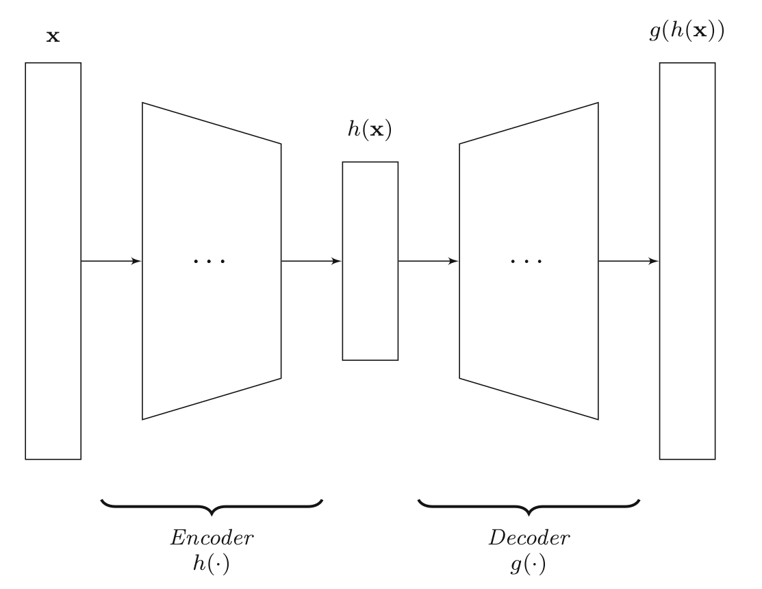
Feature extraction refers to reducing the number of dimensions in a data point so that it is computationally feasible and effective to learn a model. If we take our inputs as images of size 264x264 , we are talking about input size of 69696 pixel values, which is computationally very expensive and training a model can take very long. Hence we need to reduce the input size to a practical lower-dimensional feature vector keeping in mind that we do not lose the most important aspects of the image. This is the basic principle of feature extraction.

The figure above shows a simple encoder-decoder network that helps in learning important features from our input vectors. These are referred to as Autoencoders and are useful in finding a lower-dimensional representation of the input space without sacrificing substantial amount of information. Feature extraction is very important in Computer Vision and Natural Language Processing (NLP) applications. You can find a lot of methods that use convolutional neural networks for feature extraction from unlabeled data.
Cluster-then-label Methods
As clear by the name, cluster-then-label approaches form a group of methods that explicitly join the clustering algorithm to available data, and use the resulting clusters to guide the classification process. The main principle is to combine unlabeled data (only a subset sometimes) with the labeled data and cluster them together. A classifier is then trained independently for each cluster on the labeled data contained in it. Finally, the unlabeled data points are classified using the classifiers for their respective clusters.
Goldberg et al. in 2009, proposed to cluster the data points by constructing a graph over the data points using some distance metric. Cluster-then-label methods are generally used to identify high-density regions in the data space which are then used to help a supervised classifier in finding the decision boundary, which overall constitutes a semi-supervised approach.
Pre-training
Pre-training is very common these days in deep learning as it helps in the initialization of weights for a model. We can see these methods in the form of deep belief networks and stacked autoencoders. These methods are aimed to guide the parameters of a network towards interesting regions in model space using unlabeled data, before fine-tuning the parameters with the labeled data. These are some popular contexts where pre-training is used in deep learning:
- Unsupervised embeddings are pre-trained and are used as inputs to NLP algorithms
- Deep Stacked denoising autoencoders are used where layer wise pre-training is done one layer at a time
- Embedding like methods are also used as pre-trained inputs in many vision tasks
3. Intrinsically semi-supervised Methods
These methods directly optimize an objective function with components for labeled and unlabeled samples and do not rely on any intermediate steps or supervised base learners. Basically, these methods are extension of existing supervised methods to include the effect of unlabeled data samples in the objective function. These methods are grouped into four categories based on the underlying assumption of the data (as we learned at the beginning of this post).
For instance, maximum-margin methods rely on the low-density assumption where as perturbation-based methods directly incorporate smoothness assumption. The third category is manifold-based which either explicitly or implicitly approximates the manifolds on which the data lie. Finally, we also consider generative models.
Maximum-margin Methods
Maximum-margin classifiers attempt to maximize the distance between the given data points and the decision boundary (as considered in low-density assumption), i.e. the decision boundary must be in a low-density region of the data space. Thus, we can incorporate knowledge from unlabeled data to determine where the density is low and thus, where a large margin can be achieved.
The most prominent supervised methods that imply this principle are Support Vector Machines (SVMs), Gaussian Processes, and Density Regularization. For instance, the objective of an SVM classifier is to find a decision boundary that maximizes the margin, where margin is defined as the distance between the decision boundary and the data points closest to it. We kind of get the gist of what these methods probably tend to achieve. If you would like to know more about margin methods, and their applications in NLP, you can refer to this slide from UC Berkeley here.
Perturbation-based Methods
Perturbation simply stands for causing uneasiness or unsettling something and perturbation-based methods rely on the smoothness assumption that assumes that a small amount of noise incorporated in data points should not affect the predictions of the classifier. These methods are often implemented with neural networks. The primary reason why perturbations or randomness (with noise) is critical is that it relates to cognitive diversity. In fact, for a deep neural network to converge, we randomly initialize the model weights at the start of the training. The entire idea of stochastic gradient descent (SGD) is to perturb the entire network (from top-down) so that it evolves towards satisfying its fitness function.
In recent days, we see Generative Adversarial Networks (GANs) performing really well as the fitness function of the network is also a trained neural network (the Discriminator). All that a GAN does is make use of random noise to generate data and learn a objective function from it without the use of any labeled data. You can refer to this paper for an in-depth analysis of perturbations in adversarial networks.
Instead of explicitly perturbing the input data, one can also perturb the neural network model itself. We can compare the activations of the unperturbed parent model with those of the perturbed models in the cost function as mentioned in the work by Bachman et al. in 2014. In the semi-supervised context, if deeper layers in a deep neural network can increasingly express abstract representations of the input sample, one can argue that unlabeled data could be used to guide the network towards more informative abstract representations. One such approach is the ladder network, proposed by Rasmus et al. in 2015 which extends a feedforward network to incorporate unlabeled data by using the feedforward part of the network as the encoder of a denoising autoencoder, adding a decoder, and including a term in the cost function to penalize the reconstruction cost. Similarly, there are other methods such as \(\pi\)-model, temporal ensembling, mean teacher, and virtual adversarial training.
Manifolds
As seen in perturbation-based methods, adding slight changes in the input works well for the network to learn under smoothness assumption, but it is not the case for all cases. In some low-dimensional datasets, not all minor changes to the input should yield similar outputs. One can expect the classifier to be insensitive only to minor changes along the same manifold. Therefore, using the property of manifold assumption, methods can make changes in the data which are in the same manifold. There are mainly two different methods under this assumption. Firstly, we consider manifold regularization techniques, which define a graph over the data points and implicitly penalize differences in predictions for data points with small geodesic distance. Secondly, we consider manifold approximation techniques, which explicitly estimate the manifolds on which the data lie and optimize an objective function accordingly.
Generative Models
One of the primary goals of generative models is to model the process (or method) that generated the data. When such model is fine-tuned on a data with label y, it can also be used for classification. There are different types of generative models such as Mixture Models, Generative Adversarial Networks (GANs), Variational Autoencoders, etc which try to model a function that can be useful in generating similar data from random noise. These methods have become very popular recently and are used a lot in deep learning research for computer vision. These models make use of unlabeled data to learn the underlying relationship between random noise and the available data. Integrating these models to your network can bolster the performance of any classification method as it helps in extracting the most useful information from the input.
Conclusion
This concludes a brief overview of categorization of semi-supervised methods that follow inductive learning. Another approach as discussed earlier, that follows trasductive learning are generally represented as graph-based methods and is out of the scope for this post. The most notable techniques to take-away from this post are the recent advancements in semi-supervised neural networks, which are generally perturbation-based. They incorporate the relatively weak smoothness assumption and have shown to consistently outperform their supervised counterparts.
